Forward propagation of errors through time

TL;DR We investigate a fundamental question in recurrent neural network training: why is backpropagation through time always ran backwards? We show, by deriving an exact gradient-based algorithm that propagates error forward in time (in multiple phases), that this does not necessarily need to be the case! However, while the math holds up, it suffers from critical numerical stability issues as the network forgets information faster. This post details the derivation, the successful experiments, an analysis of why this promising idea suffers numerically, and the reasons why we did not investigate it further.

Do we necessarily need to calculate error signals in backward time (as in backpropagation through time) when training recurrent neural networks? Surprisingly, no.

In this post, we derive a method to propagate errors forward in time. By using a “warm-up” phase to determine initial conditions, we can reconstruct the exact error gradients required for learning without ever moving backward through the sequence. This sounds like a perfect solution for neuromorphic or analog hardware and a potential theory for how our brains learn, as we no longer suffer from the huge memory requirements of backpropagation through time and its to reverse the time arrow.

However, there is a catch.

While we successfully trained deep RNNs using this method on non-trivial tasks, it suffers from a critical flaw that prevents it from being widely applicable. The algorithm suffers from severe numerical instability whenever the neural network is in a “forgetting” regime. Essentially, the math works, but the floating-point arithmetic does not.

Despite these negative results, we decided to report our findings through this blog post, as we learned a lot on the fundamentals of backpropagation through time, an algorithm that is at the core of deep learning. While not directly applicable, we hope that the ideas we discuss here may sparkle some new ones and that it may be useful for the search of alternative physical compute paradigms!

---

---

Backpropagation of errors through time

Before diving into how we can propagate error signals in time, let us review backpropagation through time (BPTT) and why we would like to improve upon it in the first place.

Notation and derivation

We consider a recurrent network with hidden state $h_t$ that satisfies $h_0 = 0$ and evolves according to the following dynamics:

\[\begin{equation} h_t = f_\theta(h_{t-1}, x_t) ~~~\mathrm{for}~ t=1 \text{ to } T \end{equation}\]

The loss $L$ measuring the quality of the hidden states is defined as:

\[\begin{equation} L = \sum_{t=1}^T l_t(h_t) \end{equation}\]

where $l_t$ is the time-dependent loss function, which depends on e.g. the current target $y_t$ if we are in a supervised learning regime, and some readout weights transforming the hidden state into predictions. For the derivations that will follow, we require that this $l_t$ term has no internal memory; in particular, this means that it cannot represent a recurrent network (a feedforward one is fine) and that there is no need to propagate errors signal through time for this term.

We have now everything needed to derive the backpropagation equations. We first introduce the error term

\[\begin{equation} \delta_t := \frac{\mathrm{d} L}{\mathrm{d} h_t}^\top, \end{equation}\]

which captures how the hidden state at a given time influence the loss. If we know these error terms, we can directly compute the gradient of the loss:

\[\begin{equation} \frac{\mathrm{d} L}{\mathrm{d} \theta} = \sum_t \frac{\mathrm{d} L}{\mathrm{d}h_t} \frac{\partial h_t}{\partial \theta } = \sum_t \delta_t^\top \frac{\partial f_\theta}{\partial \theta}(h_{t-1}, x_{t}). \end{equation}\]

Note that we use $\mathrm{d}$ to denote total derivatives and $\partial$ for partial derivatives. Now, we are left with computing the errors. The standard way (which we will show can be changed!) to derive them is to

1. Remark that $\delta_T$ is easy to compute, as $\delta_T = \mathrm{d}_{h_T} L^\top = \partial_{h_T} l_T^\top$, which only requires information directly available at time $T$.
2. Remark that we can easily compute $\delta$ recursively starting from $T$ to $1$, as applying the chain rule gives

\[\begin{equation} \delta_{t} = \frac{\partial f_\theta}{\partial h}(h_t, x_{t+1})^\top \delta_{t+1} + \frac{\partial l_t}{\partial h_t}^\top = J_{t}^\top \delta_{t+1} + \frac{\partial l_t}{\partial h_t}^\top \label{eq:bptt} \end{equation}\]

where we introduced $J_t := \partial_hf_\theta (h_t, x_{t+1})$ to be the recurrent Jacobian.

The problem with backpropagation through time

While backpropagation through time works perfectly fine for most modern learning applications, it suffers from a fundamental problem. To calculate the gradient at time $t$, the algorithm must first wait time $T$ for the entire sequence to be done, and then process the data in reverse order.

This retrospective property creates two issues:

1. Memory constraints: We must store the history of all hidden states to compute gradients during the backward pass. For long sequences, this memory footprint grows linearly with time, becoming prohibitive for memory-constrained systems or streaming data.
2. Biophysical implausibility: Backpropagation’s requirement to reverse the arrow of time makes it an unlikely candidate for explaining biological learning¹1. Lillicrap & Santoro, Backpropagation through time and the brain, Current Opinion in Neurobiology, 2019. or for implementation on neuromorphic hardware.

The canonical forward-mode alternative to backpropagation is real-time recurrent learning²2. Williams & Zipser, A learning algorithm for continually running fully recurrent neural networks, Neural Computation, 1989. (RTRL). Rather than propagating errors backward, it propagates sensitivities forward. These sensitivities capture how hidden states depend on parameters, can be updated alongside the hidden state, and can be used to compute gradients at any time steps.

Unfortunately, the vanilla version of this algorithm is intractable because of its memory (cubic in the number of hidden neurons) and computational (quartic in the number of hidden neurons) complexities.

Approximations have been introduced to make it tractable. They typically involve operating as if recurrent connectivity was diagonal^3,3. Bellec et al., A solution to the learning dilemma for recurrent networks of spiking neurons, Nature Communications, 2020.⁴4. Murray, Local online learning in recurrent networks with random feedback, eLife, 2019. (thus considerably reducing complexity and being exact when connectivity is diagonal⁵5. Zucchet, Meier, Schug, Mujika & Sacramento, Online learning of long-range dependencies, NeurIPS, 2023.), or performing random low-rank approximations^6,6. Tallec & Ollivier, Unbiased online recurrent optimization, arXiv:1702.05043, 2017.⁷7. Mujika, Meier & Steger, Approximating real-time recurrent learning with random Kronecker factors, NeurIPS, 2018. of the sensitivity matrix. Additional approximations must be introduced for deep recurrent networks, that implicitly ignore all the downstream recurrent layers when computing gradients.

To summarize: there is definitely some room for improvement between backpropagation through time (exact, but offline) and real-time recurrent learning (online, but has to be approximated to be practical most of the time). Ideas on how to achieve that are currently missing, the following will be a small step in that direction.

Forward propagation of errors through time (FPTT)

Let us now move to the meat of this blog post: how we can do forward propagation of errors through time. This will rely on two main insights: in most cases we can invert the backpropagation equation and compute $\delta_{t+1}$ from $\delta_t$, and a warm-up forward pass can provide us with the initial condition from which we can start (re)constructing the errors trajectory. Let us unpack this.

Insight 1: Inverting the backpropagation equation

The backpropagation equation (Equation $\ref{eq:bptt}$) defines a linear system of equations. It is most natural to use it to compute $\delta_t$ as a function of $\delta_{t+1}$, but nothing forbids us from inverting that system (when $J_t$ is invertible of course!) to compute $\delta_{t+1}$ from $\delta_t$; we get:

\[\begin{equation} \delta_{t+1} = J_t^{-\top} \left (\delta_t - \frac{\partial l_t}{\partial h_t}^\top\right). \label{eq:fptt} \end{equation}\]

In particular, this means that if we know the correct value of $\delta_0$ (which is not obvious a priori!) and we run this equation as we process the input sequence, we will get the exact error trajectory that is needed in the gradient calculation.

But how do we get that?

Insight 2: a warm-up forward pass to initialize the error dynamics

To compute the initial $\delta_0$ that will enable forward propagation of error through time, we will leverage a property of time-varying linear dynamical systems (which Equation $\ref{eq:fptt}$ is an example): the difference between two trajectories starting from different initial conditions evolves according to a simple formula that only depends on the initial conditions and the product of time-varying matrix:

\[\begin{equation} \delta'_T - \delta_T = \left ( \prod_{t'=0}^{T-1} J_{t'}^{-\top} \right ) \left (\delta'_0 - \delta_0 \right ). \end{equation}\]

In the previous equation, $\delta$ and $\delta’$ are two “error” trajectories that follow Equation $\ref{eq:fptt}$. This formula can be derived recursively:

\[\begin{equation} \begin{split} \delta'_{t+1} - \delta_{t+1} &= J_t^{-\top} \left (\delta'_t - \frac{\partial l_t}{\partial h_t}^\top\right) - J_t^{-\top} \left (\delta_t - \frac{\partial l_t}{\partial h_t}^\top\right)\\\\ &= J_{t}^{-\top} \left (\delta'_t - \delta_t \right). \end{split} \end{equation}\]

Why is this formula useful? Given that we know $\delta_T$ (see the backpropagation section), running a warm-up trajectory starting from $\delta’_0=0$ to obtain $\delta’_T$ provides us with enough information needed to compute $\delta_0$:

\[\begin{equation} \delta_0 = \left ( \prod_{t'=T-1}^{0} J_{t'} \right ) (\delta'_T - \delta_T) + \delta'_0 = \left ( \prod_{t'=T-1}^{0} J_{t'} \right ) \left (\delta'_T - \frac{\partial l_T}{\partial h_T}^\top \right ). \end{equation}\]

Remember that once we have this $\delta_0$ (which we could have also computed with backpropagation through time), we can reconstruct the exact error trajectories running the procedure described in the last paragraph.

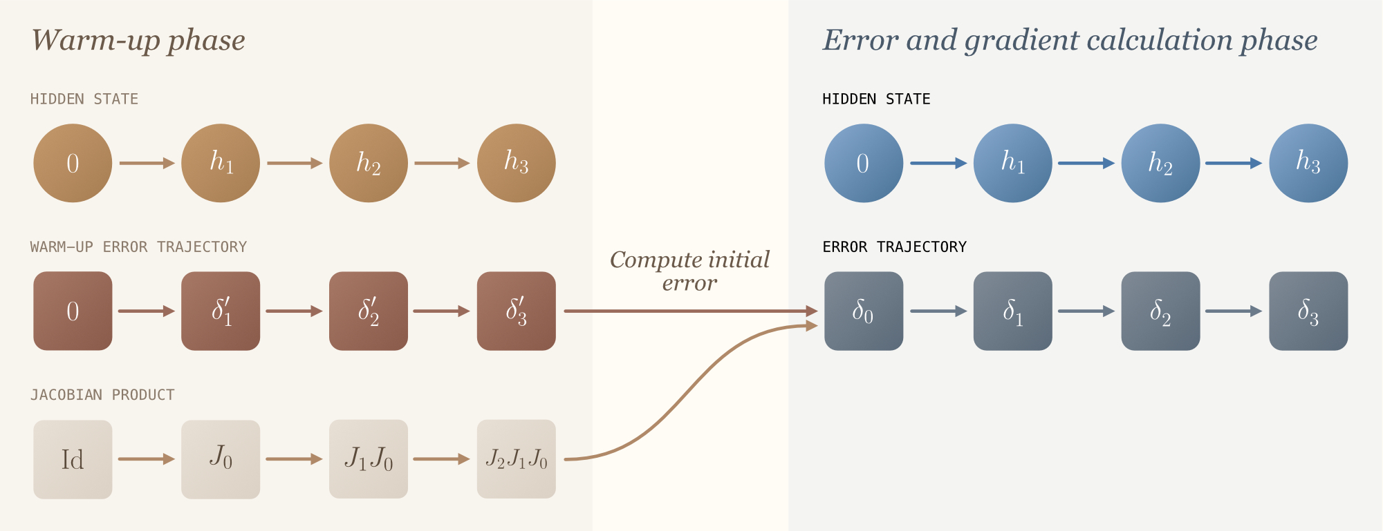
We now have everything in our hands to derive the forward propagation of errors through time (FPTT in short) algorithm:

1. Warm-up phase
   Initialize $J := \mathrm{Id}$ (to accumulate the product of Jacobians), $h_0=0$ and $\delta’_0 =0$. Process the input sequence and recursively update
   • $h_t = f_\theta(h_{t-1}, x_t)$
   • $\delta’_{t+1} = J_t^{-\top} \left (\delta’_t - \frac{\partial l_t}{\partial h_t}^\top\right)$
   • $J = J J_t$

   Compute $\delta_0$ using the formula $\delta_0 = J \left (\delta’_T - \frac{\partial l_T}{\partial h_T}^\top \right )$

2. Error and gradient calculation phase
   Initialize $h_0=0$ and $\delta_0 = 0$. Process the input sequence and recursively update
   • $h_t = f_\theta(h_{t-1}, x_t)$
   • $\delta_{t+1} = J_t^{-\top} \left (\delta_t - \frac{\partial l_t}{\partial h_t}^\top\right)$
   • the parameters in the direction of $\partial_\theta f(h_{t-1}, x_t)^\top \delta_t$.

The inner workings of the algorithm are depicted below.

The algorithm has interesting connections with shooting methods⁸8. Ascher & Petzold, Computer Methods for Ordinary Differential Equations and Differential-Algebraic Equations, SIAM, 1998. used for the numerical simulation of ordinary differential equations with boundary conditions at the final time step. The idea is to guess the initial values, run the differential equation until the final time step, compare it with the desired value, correct initial conditions, and so on. The forward propagation of error algorithm can thus be understood as a shooting method in which estimating $J$ provides an exact way to “guess” the correct initial value. Additionally, we could tweak the algorithm to estimate $\delta_0$ without having to keep track of $J$ (thus considerably reducing memory), but at the price of more forward passes.

One last thing: how do we deal with multiple layers?!

The attentive reader will have noticed that the algorithm we described does not really handle the multiple layer case.

Sure, one could consider all hidden states in a deep recurrent network to be in the same “layer”, but this creates huge Jacobian matrices (which model interlayer connections) and this is not really scalable.

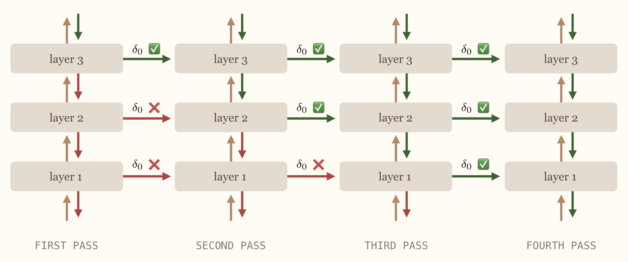
Instead, we could backpropagate errors through each recurrent layer at a time, which is also what automatic differentiation frameworks do under the hood. However, to keep things online, we will have to run multiple passes, more precisely $L+1$ if $L$ is the number of recurrent layers.

The intuition is as follows.

Let us look at the last layer, that is layer $L$. In the first warm-up pass, it computes dummy error signals, which means that it cannot provide good learning signals to recurrent layer $L-1$. However, during the second pass, we can instantaneously backpropagate the error signal that was just calculated (and which is an exact gradient) to the previous layer. This can thus be used to instantiate the warm-up phase of layer $L-1$.

More generally, we will be able to perform the warm-up phase of layer $l$ whenever layer $l+1$ is in error calculation phase, hence the $L+1$ number of passes required.

The procedure is illustrated below.

The forward propagation of error algorithm has a memory complexity that is independent of sequence length (contrarily to BPTT) and grows quadratically with the number of hidden neurons (vs. linearly for BPTT and cubic for RTRL), with the bottleneck being the accumulation of Jacobians. The main computational challenges are the computation of the entire recurrent Jacobian and its inversion, although this problem would not arise in continuous time⁹9. In continuous time, the recurrent Jacobian takes the form $J_t = \mathrm{Id} + A_t \mathrm{d}t$ where $A_t$ is the dynamics’ Jacobian and $\mathrm{d}t$ is the discretization step. As $\mathrm{d}t \to 0$, a first-order expansion gives $J_t^{-\top} \approx \mathrm{Id} - A_t^\top \mathrm{d}t = 2\mathrm{Id} - J_t^\top$, replacing the matrix inversion with a simple subtraction..

Algorithm	Memory	Number of passes (forward / backward)	Exact
BPTT	$LNT$	$1 / ~1$	Yes
RTRL	$(LN)^3$	$1 ~ / ~ 0$	Yes
Diag RTRL	$LN^2$	$1 ~ / ~ 0$	No
FPTT	$LN^2$	$L+1 ~ / ~0$	Yes

As a side note, one can see the number of forward passes a knob that we can control to improve gradient quality: the more passes we do the better the gradient quality. The forward error propagation algorithms therefore trades off compute for gradient quality, which is not something other algorithms can do precisely.

It works!…

Let’s first start with the good news.

The forward propagation of error through time can, as we will show, successfully train deep recurrent networks on relatively challenging sequential learning tasks.

Task (sequential MNIST) and model (deep linear recurrent unit)

To this end, we study a simplified version of the sequential MNIST task, which we term MNIST98. In this variant, every group of $8$ pixels is averaged together, resulting in a shorter sequence length ($98$ time steps, to make simulations faster) while maintaining the task’s inherent difficulty.

The architecture we consider consists of $4$ layers, each comprising a linear recurrent unit¹⁰10. Orvieto et al., Resurrecting recurrent neural networks for long sequences, ICML, 2023. (i.e. some recurrent layer) as well as a multi-layer perceptron (which is the non-recurrent part) — this has become the standard for powerful recurrent architectures in the last years. Note that the linear recurrent unit uses diagonal linear connectivity so aggregating and inverting Jacobians is an easy task here.

To ensure that the network faces non-trivial learning challenges and has to learn to tweak its memory, we set the number of recurrent hidden neurons to $32$ per layer (far below the $98$ time steps). We train all networks using AdamW optimization with a weight decay of $0.01$ applied to all parameters except the recurrent ones, employ a cosine learning rate scheduler, and clip gradients to a maximum norm of $1$.

We tune three key hyperparameters in this type of experiments: the learning rate, $r_{\min}$ (the minimal value the eigenvalues of the LRU can take, in ${0.9, 0.99}$) and the recurrent learning rate factor (in ${0.25, 0.5, 1}$). The latter is a standard practice in deep state-space models and involves reducing the learning rate specifically for recurrent parameters. For each hyperparameter configuration, we use $3$ different random seeds and tune the base learning rate using a logarithmic grid with base $3$ to optimize validation loss.

Results

We first compare different learning algorithms: forward backpropagation through time, standard backpropagation through time (which serves as an upper bound on performance), and spatial backpropagation (which does not propagate gradients through recurrent connections; it should provide a lower bound). A real-time recurrent learning baseline is missing from this comparison, but it would constitute a strong contender in this regime, in particular because of the diagonal structure of the recurrence⁵. The results shown below highlight that the forward propagation of errors algorithm can be a competitive learning algorithms!

Algorithm	Test loss $\downarrow$	Test accuracy $\uparrow$
Spatial BP	$0.731$	$96.55\%$
BPTT	$0.691$	$98.30\%$
FBPTT	$0.673$	$98.19\%$

These results look promising; the natural next step in a research project would be to scale things. However, we digged deeper into those results before doing so, and we found that the algorithms suffers from fundamental instabilities that we do not know how to solve with the current deep learning machinery, so we ultimately decided not scaling things up. Let us see why.

It works! but it is extremely sensitive

Looking deeper into the results of the previous section, we found that forward backpropagation of errors work significantly better when eigenvalues of the recurrence are initialized close to $1$, and when they have a small learning rate, which is not necessarily the case for backprop. This is pointing towards the fact that the algorithm requires eigenvalues to be in a specific range to work properly. In the following we investigate this question in a controlled environment, as well as provide theoretical arguments for why this is the case.

Trained networks must not forget

In this section, we will consider a single layer of linear recurrent units and compare the gradients numerically obtained with FPTT vs. the one with BPTT. This architecture is particularly handy for our purposes as this is the one we used in the previous section, but also it enables precise control over the eigenvalues of the recurrent Jacobian, which will be an important quantity here.

More precisely, we vary the $r_\mathrm{min}$ factor we used in the previous section and observe how the gradient quality evolves. We find that gradient quality quickly deteriorates if $r_\mathrm{min}$ is too small, and that increasing the sequence length makes that trend even worse, cf. figure below.

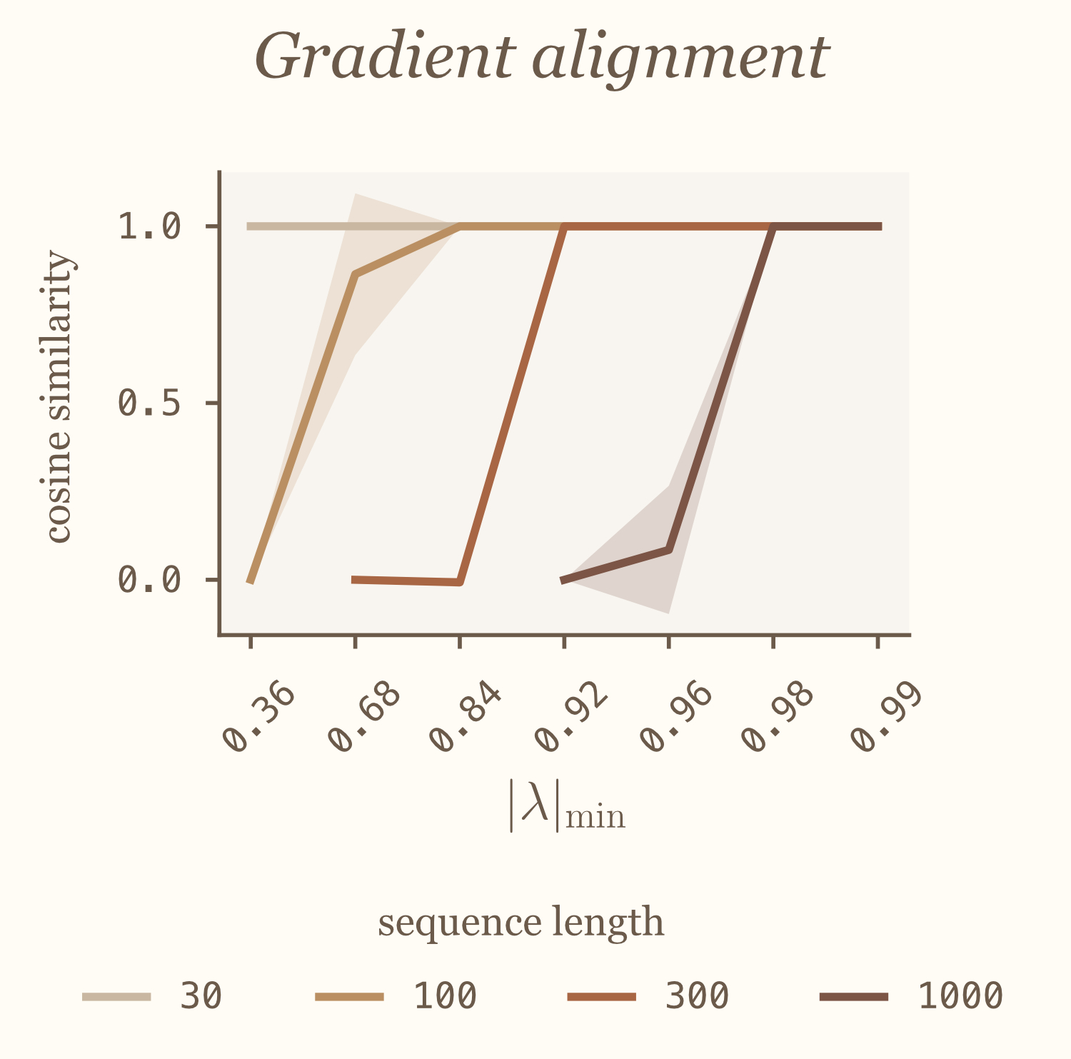
That is, for FBPTT to work, we need the eigenvalues of the Jacobian to be above some threshold for things to be well behaved. Networks that forget cannot be learned with our forward propagation of error algorithm.

Why forgetting hurts forward propagation of errors?

Let us try to understand the reasons behind what we just observed. For that, we will draw intuition from dynamical systems theory.

A linear dynamical system is said to be stable if the eigenvalues of its transition matrix have modulus smaller than $1$. Such stable systems have the following properties: their state remains bounded if their inputs are bounded, and initial conditions are forgotten exponentially fast. When this condition on the eigenvalues of the recurrent transition matrix is not satisfied, we can observe exponentially exploding behavior.

Similar intuition holds for time-varying and nonlinear dynamical systems (one needs to introduce the notion of contractivity to properly handle this case, but this will be for another time).

This stable regime is typically the one in which we want to operate when training recurrent neural networks, as it avoids explosion of the forward pass. As a consequence, the backpropagation equation (Equation $\ref{eq:bptt}$) will also be stable. However, the forward propagation of error will not! This is because we invert the Jacobian, so eigenvalues with modulus smaller than 1 become eigenvalues with modulus greater than 1.

Contractive recurrent networks (which we want) will therefore yield exploding forward propagation of errors (which we don’t want). Indeed, warm-up errors and the product of inverted Jacobians might diverge exponentially fast, and finite numerical precision is not sufficient to accurately capture gradient information. This will create approximations to $\delta_0$, which will further get amplified in the error calculation phase.

Let us now get some more quantitative understanding of this effect, by studying the simplest (but powerful¹¹11. Zucchet & Orvieto, Recurrent neural networks: vanishing and exploding gradients are not the end of the story, arXiv:2405.21064, 2024.!) case: the 1D linear case, that is $h_{t+1} = \lambda h_t + x_{t+1}$ with $\lambda$ the recurrent parameter (and Jacobian). If we have an initial imprecision of $\varepsilon$ on $\delta_0$, this imprecision will become $\lambda^{-T} \varepsilon$ at the end of the sequence, which exponentially diverges (as $\lvert\lambda\rvert < 1$). This explains why we observed that longer sequences require larger $\lvert\lambda\rvert$ to avoid accurately compute gradients, due to the amplification of errors we just described.

Given that we want to train recurrent networks at the edge of stability (to avoid vanishing and exploding gradients), is this instability of forward error propagation really that bad?

It is true that successful deep learning architectures are usually initialized in this regime. When the recurrence is linear, we will not deviate too much from this regime during learning, which is why our experiments above worked reasonably well. However, most recurrent architectures that are currently used in practice (e.g., LSTMs^12,12. Hochreiter & Schmidhuber, Long short-term memory, Neural Computation, 1997.^13,13. Beck et al., xLSTM: Extended long short-term memory, NeurIPS, 2024. Mamba^14,14. Gu & Dao, Mamba: Linear-time sequence modeling with selective state spaces, arXiv:2312.00752, 2023. Hawk^15,15. De et al., Griffin: Mixing gated linear recurrences with local attention for efficient language models, arXiv:2402.19427, 2024. Gated DeltaNet¹⁶16. Yang, Kautz & Hatamizadeh, Gated delta networks: Improving Mamba2 with delta rule, ICLR, 2025.) develop some data-dependent forgetting (i.e., eigenvalues with modulus smaller than $1$) during learning, and thus forward propagation of errors will likely run into numerical issues at some point during training.

Looking ahead

Overall, we believe that the conditions are not met (at least currently) for the forward propagation of errors to be practically useful. We review below the different reasons:

• Instability of the algorithm.
  We have discussed this in depth in the last question. Still, there are a few arguments we can add to this point. On the positive side, it may be possible to reduce the numerical instability of the system by other numerical types. For example, we found that switching float32 to float64 improves the situation, and it is likely that numerical types suited for these exponential behaviors¹⁷17. Heinsen & Kozachkov, Generalized orders of magnitude for scalable, parallel, high-dynamic-range computation, arXiv:2510.03426, 2025. might improve it even further. It may also be that we get better at developing recurrent architectures that remain at the edge of stability over the course of learning. On the flip side, this dynamical instability implies a huge dependency on initial conditions, in particular $\delta_0$. This means that it is unlikely that amortized methods that would provide a rough estimate of $\delta_0$ (to skip the warm-up phase) are good enough to yield good performance. Additionally, in cases where the recurrent Jacobian is low-rank and therefore not invertible, the algorithm simply breaks.

• Are the multiple forward passes really worth it?
  One algorithm that we have not yet discussed is the reversible backpropagation through time¹⁸18. MacKay, Vicol, Ba & Grosse, Reversible recurrent neural networks, NeurIPS, 2018.. It consists in recomputing the hidden states in the backward pass, which is possible when the update function is invertible (this is easy in continuous time, it requires some architectural tweaks¹⁹19. Gomez, Ren, Urtasun & Grosse, The reversible residual network: Backpropagation without storing activations, NeurIPS, 2017. in discrete time). If the system is Hamiltonian, it is even possible to compute errors without an explicit gradient calculation circuitry²⁰20. Pourcel & Ernoult, Learning long range dependencies through time reversal symmetry breaking, arXiv:2506.05259, 2025.. This algorithm is exact, requires two passes, and also requires storing the input, like forward backpropagation through time. It is unclear whether the multiple forward passes of forward error propagation, as well as the additional machinery required to compute Jacobian products, is worth the gains we get by having an algorithm that fully operates in forward mode.

• The cost of computing and inverting Jacobians.
  The forward propagation of errors algorithm requires computing and inverting Jacobians. Regarding Jacobian computation, there is in general no alternative to computing the full Jacobian, as one cannot use Jacobian-vector products to compute the initial $\delta_0$. This operation has cubic computational complexity and may require dedicated circuits. When the recurrent layer has a specific structure, as is the case with linear or vanilla recurrent networks, the computational footprint can be reduced. There are several alternatives when it comes to Jacobian inversion. First, as we mentioned earlier, the need for inversion disappears when moving to continuous-time systems, which is where the most promising applications of this method lie (think analog computing^21,21. Aifer et al., Solving the compute crisis with physics-based ASICs, arXiv:2507.10463, 2025.²²22. Momeni et al., Training of physical neural networks, Nature, 2025.). Second, even in discrete time, there are numerous techniques to efficiently compute inverse-Jacobian-vector²³23. Bai, Kolter & Koltun, Deep equilibrium models, NeurIPS, 2019. products by iterating over a linear system or by leveraging analog systems^24,24. Donatella et al., Thermodynamic natural gradient descent, npj Unconventional Computing, 2026.^25,25. Jang, Lee & Shin, An optimization network for matrix inversion, NeurIPS, 1987.²⁶26. Kendall, Fast target propagation for machine learning and electrical networks, US Patent App. 18/516,474, 2024..

• The input still needs to be stored in memory.
  This is a more minor point. Compared to other forward-mode algorithms like real-time recurrent learning, the forward error propagation algorithm requires storing and repeating the input sequence. In terms of absolute amount of memory, this is much better than storing the entire hidden state trajectory, but it remains a small drawback of the algorithm.

For these reasons, we have decided to not pursue further our investigations related to this algorithm. Yet, we decided to make the results of our investigations public as we learned a lot questioning why things (here backpropagation through time) are done in a certain way (here ran backwards). While not directly useful, we hope that these ideas can sparkle new ones.

---

Appendix: Time and memory complexities

We provide a more fine-grained complexity analysis of different gradient computation algorithms for recurrent neural networks. We focus on a single recurrent layer with $N$ hidden neurons for simplicity and denote, as before, the sequence length by $T$. We include reversible backpropagation through time¹⁸ in this analysis, which avoids storing the full activation trajectory by reconstructing hidden states during the backward pass (exploiting the invertibility of the recurrence), as its existence is one of the main reasons we did not scale up our experiments.

The memory, time, and memory access complexities of each algorithm are summarized below.

Algorithm	Memory	Time	Memory accesses	Passes (forward / backward)	Exact
BPTT	$NT$	$N^2T$	$NT$	$1 ~ / ~ 1$	Yes
Exact RTRL	$N^3$	$N^4T$	$N^3T$	$1 ~ / ~ 0$	Yes
Diagonal RTRL	$N^2$	$N^3T$	$N^2T$	$1 ~ / ~ 0$	No
Reversible BPTT	$N$	$N^2T$	$NT$	$1 ~ / ~ 1$	Yes
FPTT	$N^2$	$N^3T$	$N^2T$	$2 ~ / ~ 0$	Yes

A few takeaways from this comparison:

• All the alternatives to backpropagation through time listed above eliminate the linear scaling of memory with sequence length.
• Forward propagation improves over real-time recurrent learning by a factor $N$ in all complexity metrics, and has similar complexities to the diagonal approximation of RTRL.
• Reversible backpropagation dominates forward propagation of errors in all complexity metrics. It does not suffer from numerical stability issues, but it does require a backward pass and the recurrence to be invertible (a similar constraint to the one forward propagation has).